Master's Thesis:
Anti-Derivative Anti-Aliasing for the Chebyshev Non-Linear Model
A master's research project submitted to the faculty of the University of Miami in partial fulfillment of the requirements for the degree of Master of Science. Approved by Christopher Bennett (Ph.D., Department Chair), Tom Collins (Ph.D., Associate Professor), Justin Mathew (Ph.D., Adjunct Professor), and Shannon K. de l’Etoile (Ph.D., Associate Dean of Grad Studies).
Abstract
There have been many techniques for modeling static memoryless non-linearities, with the Synchronized Sine-Sweep Method in combination with the Chebyshev Non-Linear Model proving to be one of the most effective. Unlike other similar approaches such as the Simplified Volterra and Legendre models, the Chebyshev model offers a unique advantage due to its close relation to certain cosine identities, allowing for the extreme simplification of the necessary calculations. However, when modeling any non-linear system that introduces harmonics and high-frequency content, aliasing emerges as a significant and problematic issue. To combat this, a method known as Anti-Derivative Anti-Aliasing (ADAA) was developed, proving highly effective in lowering the energy of aliasing frequencies in other non-linear systems. This thesis explores the application ADAA specifically to the Chebyshev model, and defines general equations for the modified approach. It was found that the implementation of ADAA successfully reduced aliasing in two variations of the model, providing an average attenuation of 16.25 dB when measuring the first 16 aliasing harmonics of a wave-shaped 5kHz test-tone. Overall, the adapted method serves as an optimal way to emulate a non-linear system while minimizing the drawbacks of digital artifacts.
Chapter 1: Introduction
Many analog audio systems, including guitar amplifiers and tape recorders, exhibit some form of non-linear behavior that shapes the waveform of an audio signal, creating additional harmonic content that is pleasing to the ear. This concept plays a crucial part in music production, especially in genres known for their use of distortion such as rock and hip-hop. Utilizing a non-linearity in a creative setting could be as subtle as saturating the kick drum to make it more present in a mix, or as aggressive as overdriving an electric guitar to transform it into a screaming lead. However, in the era of laptop music production, digital audio workstations, and low-budget setups, the use of analog gear has become considerably less popular; and instead, producers and musicians have gravitated towards digital solutions due to their consistency, reliability, and decreased cost. Thus, as the audio industry continues to shift towards digital emulations of traditionally expensive analog gear, the ability to accurately model these analog systems and their non-linear characteristics becomes increasingly crucial.
When attempting to emulate a non-linear system without any prior information, a technique called the Synchronized Swept-Sine Method can be adopted to accurately replicate and model it. This technique is only effective for memoryless non-linearities—meaning the system does not consider previous or future values of the signal, such as a hyperbolic tangent function tanh(x) which processes only the current signal value. The approach involves first sending an exponential swept-sine excitation signal through the system, whose output is then deconvolved with the original input sweep. This results in individual impulse responses (IRs) containing information specific to each harmonic created by the non-linearity, separated by a time gap. The separation is advantageous, as it allows for information from each impulse response to be utilized separately during processing.
Each impulse response relates to the multiple harmonics of the signal—the first IR holding information for the first order, cos(θ), then the second harmonic cos(2θ), then the third harmonic cos(3θ), and so forth. To model and replicate these harmonics, however, they need to be related to operators that can be applied to a digital audio sample of a signal, such as x^2, x^3, x^4, and so on. Researchers have previously found methods for achieving this relation between 2θ, 3θ, 4θ … and x^2, x^3, x^4 …, with the most popular techniques utilizing a “mixing matrix,” where the Discrete Fourier Transform (DFT) of each impulse response is used to calculate coefficients for x^2, x^3, x^4 … or multipliers for increasing orders of a polynomial series. These calculations for the mixing matrix need to be completed beforehand, which can be quite complex and time consuming; however, once these coefficients are found, the digital input sample x can be processed with simple power operators to model the original non-linear system. As discussed in more detail in chapter 3, the use of Chebyshev Polynomials of the First Kind provides a much simpler way of modeling a non-linear system when compared to other polynomial series, as it allows for each impulse response extracted from the Synchronized Swept-Sine Method to be directly implemented as FIR filters, via discrete time convolution. Thus, there is no need for a mixing matrix, and the complex calculations that are required to create it. This is called the Chebyshev Model.
When digitally modeling systems, particularly those that generate potentially infinite harmonics like a memoryless non-linearity, aliasing is a significant concern. In simple terms, aliasing distortion occurs when a frequency exceeds what the digital sampling rate can accurately capture, resulting in an inaccurate representation of the original signal. This is fundamentally different than the pleasant distortion introduced by a non-linear system, since aliasing frequencies are not harmonic or musically related in any way; instead, aliasing distortion creates sounds that are jarring and out of place. To combat this, a method known as Anti-Derivative Anti-Aliasing (ADAA) was developed by Julian Parker et al. in [14], which has proven to be effective in decreasing the energy in aliasing frequencies considerably in non-linear systems. More recently, ADAA has been applied to other non-linear models such as the Simplified Volterra model, shown in a recent paper written by C. Bennet and S. Hopman [11]. When compared to popular anti-aliasing methods such as oversampling, ADAA can serve as a more efficient alternative in certain applications. This approach also proves to be beneficial for the Volterra Model, since significant phase shifts from a traditional low-pass filter could cause the system to break.
Put simply, the ADAA method for reducing aliasing is done by first creating a continuous-time version of the signal using interpolation between samples. The non-linearity is then applied, followed by a lowpass filter kernel in continuous-time to lower the amplitude of aliasing frequencies. The signal is sampled again at the original sample rate, creating the anti-aliased digital signal. This special process allows for the derivation of an analytical solution, which is relatively straight-forward to implement and understand. This paper investigates the application of ADAA to the Chebyshev Non-Linear Model, evaluating its effectiveness in reducing aliasing in this specific context. This requires the development of a new method, as the structure of the Chebyshev Model is fundamentally different than other non-linear modeling techniques and thus requires a unique structure for supporting ADAA.
Ultimately, the Chebyshev Non-Linear Model combined with ADAA shows promise for achieving the much-desired harmonic distortion effect sought by musicians and producers alike, while minimizing the unwanted and unpleasant distortion caused by aliasing and limitations of digital audio. Therefore, this project serves as a stepping-stone in making emulations of expensive analog gear and their non-linear behavior more accurate, effective, and accessible to all.
Chapter 2:
The Synchronized Swept-Sine Method

Figure 1: Synchronized Swept-Sine HHIR Extraction
The Synchronized Swept-Sine Method is a technique for extracting information for each harmonic created by a memoryless non-linear system, in the form of individual impulse responses. Each individual IR, denoted h(t) in (fig. 1), contains the frequency and phase response for its respective kth multiple harmonic sin(kθ) introduced by the non-linear device under test. In Antonin Novak’s paper [1], he calls these IRs “Higher-Harmonic Impulse Responses,” or HHIRs for short, which can then be further processed to create an estimation of the original non-linear system. Thus, the approach is particularly useful for creating a digital emulation of a system where the non-linear nature is unknown, such as a guitar amplifier or distortion pedal.
In this chapter, an overview of the Synchronized Swept-Sine Method is given as outlined by Novak in [1], along with an introduction to a similar cosine-sweep method.
2.1 Sine Sweep
A Synchronized Swept-Sine can be characterized as:

which is used as the excitation signal for the device under test. L is the rate of frequency increase for the sweep, defined as:

where f1 and f2 represent the desired start and stop frequencies, T̂ represents the desired approximate time duration of x(t), and “round” represents a rounding function to the nearest integer. When looking at Novak’s paper [1], his equation defining includes a “-1” term in the expression to fix the initial phase of the sweep, but differs from equation (1) shown above; but as he explains later in the paper, the omittance of “-1” yields the exact same result since the round function in equation (2) ensures f1L is always an integer.
To better understand its significance, Novak explains the special process of calculating L and the use of a rounding function is mainly to keep the phase of the sweep x(t) fixed at zero for t=0, as any deviation of can result in phase estimation issues of the HHIRs. This initial fixed phase can also be notated with the equation φ(0) = 2πk, which states the phase φ at time 0 must be a k multiple of the period 2π, ensuring the sweep starts at the beginning of a period. Since a sine function is used for the sweep, the signal will start with a value of zero, since sin(2πk) = 0. Novak then uses the following equation for k:

where T is the actual time of sweep x(t), and k is a non-zero integer. Since the ability to define and change the start frequency, stop frequency, and time duration of the sweep is desired, an issue arises; there are only very specific combinations of these three parameters where k is an integer, and many inputs of f1, f2, and T will result in a non-integer value. In practice, this issue can be avoided by using the round function as shown below:

where now T̃ represents a desired estimation of the time duration T, and L = k/f1 in accordance with equation (2). With this approach, one can define and change the variables f1, f2, and T̃ as they please, all while ensuring k is an integer. The actual duration of the sweep T will deviate slightly from T̃ when using this method, so its value can be derived by combining equations (3) and (4) if needed.

The sweep x(t) has a unique property that allows for the extraction of the HHIRs, where shifting the synchronized swept-sine signal by a time gap Δtk results in the kth higher harmonic copy of x(t) itself. Here, Δtk = L ln(k) as defined in [1].

Figure 2: Synchronized Swept-Sine Time Alignment
To help understand why this is important, one can use the following example shown above in (fig. 2): two identical copies of the sine sweep are made, which can be labeled as x1 and x2. If one were to overlap these sweeps so that an instantaneous frequency in x1 (say 1kHz, for example) were to line up with double that frequency in x2 (2kHz, in this case), then, all instantaneous frequencies in x1 will be aligned with double its frequency in x2. So, the 200Hz place in x1 will be aligned with 400Hz in x2, and 7.5kHz in x1 will be aligned with 15kHz in x2, and so on. This holds true for any multiple as well; if one were to align the two sweeps so that an instantaneous frequency in x1 (say 1kHz) were to align with triple that frequency in x2 (3kHz in this case), then all instantaneous frequencies in x1 will be aligned with triple its frequency in x2. This synchronization is crucial, as it allows for all the harmonic multiples introduced by the non-linear system to be aligned during deconvolution.
Once the sine sweep x(t) is ran through the non-linear system, the resulting output of the system can be denoted as y(t), which will simply be a wave-shaped version of x(t) containing its harmonics. Now, any place in y(t) (1kHz place, for example) will also contain its multiple harmonics (2kHz, 3kHz, 4kHz …). So with the property discussed above, the output y(t) can just be thought of as an addition of multiple copies of x(t) with different time offsets Δtk.

Figure 3: Harmonic Composition of y(t)
Being able to treat each harmonic of the signal separately allows us to later determine how much of each harmonic is created from the non-linear system; and once this information is obtained, the process of modeling the non-linearity becomes significantly more straight-forward.
2.2 Deconvolution
To extract the information regarding each harmonic of the signal, the non-linear system’s output must be de-convolved with the original excitation signal. The deconvolution process can be seen as a way to remove the original sine sweep x(t) from the device’s output y(t), leaving only harmonic information in the form of individual IRs. Since there is no real “deconvolution” operation in the time domain, a special process must be used to achieve this result. One such method is to convolve x(t) with its “inverse signal” as outlined in [2], which successfully accomplishes the deconvolution process. This starts with the creation of an analysis signal z(t), which can be thought of as the “exact opposite” or inverse of the sweep x(t). This analysis signal is a time reversal of the sine sweep and has an amplitude envelope of -10dB/decade, which compensates for the exponential frequency increase that causes x(t) to have considerably more energy in the lower range. This results in a signal that decreases in frequency over time, and resembles the following:

Figure 4: Resemblance of Analysis Signal, z(t)
To properly construct this analysis signal z(t), the original sine sweep is first converted to the frequency domain using the Fourier Transform, where the inverse is created (1/H(ω)). A band-pass filter is applied at the beginning and end frequencies to prevent noise amplification, and then the Inverse Fourier Transform is performed to convert the signal back to the time domain. This process ensures that the analysis signal z(t) has phase and magnitude characteristics that that are complementary to x(t).
The output of the non-linearity y(t) and analysis signal z(t) can now be convolved using discrete-time convolution, which first involves z(t) being time-reversed again, yielding z(-t). The reversed signal now resembles x(t) exactly, other than the amplitude envelope; and the rest of the convolution process then determines the points of correlation, or similarity, between the two signals.

Figure 5: Extraction of HHIRs using Discrete-Time Convolution
As a review, the process of discrete-time convolution involves lining up the last digital sample of z(-t) with the first sample of y(t), then multiplying each overlapping sample value (only one overlap, in this case), and adding all the products together—which results in the first output value of the convolution operation. After this is completed, z(-t) is then “slid” to the next sample, so now two samples are overlapping with y(t), and the process repeats; each sample value in z(-t) is multiplied with the overlapping sample in y(t) and all the products are added together, resulting in our second output value of the convolution operation. This is repeated until z(-t) is slid all the way to the end, where the only overlap is the last sample of y(t) with the first sample of z(-t). So, when there is some similarity between the two signals, a “spike” will show up in the output of the convolution—or more formally known as an impulse response. Since the presence of a harmonic in y(t) can be thought of as simply the addition of another copy of x(t) with a time gap as outlined in (fig. 3), a spike will occur every time the analysis signal is offset by Δt1, Δt2, Δt3 … and so on. The shifting of the time-reversed analysis signal starts with the longest time-gap, Δtk, which means that the first impulse response to show up in the convolution output would be hk(t) corresponding with the highest harmonic. As the analysis signal shifts, the time gap becomes smaller, meaning the harmonic impulse responses will show up in the output in decreasing order. This continues until y(t) and the analysis signal are overlapped entirely, which results in the last impulse response h1(t) representing the 1st harmonic (fundamental).
2.2 A More Practical Approach
The deconvolution process can also be achieved with a simple division operation in the frequency domain, which is a far more practical approach during implementation when compared to the time-domain method outlined above (although, the previous method is important for understanding how the impulse responses are extracted during deconvolution). The process of extracting all impulse responses h(t) can now be defined as:

Where X(f) and Y(f) are the frequency-domain equivalents of x(t) and y(t), respectively. Y(f) can be obtained by simply taking the FFT of y(t), and the Fourier Transform of the swept sine x(t) is defined for positive frequencies from [1] as:

The division of X(f) and Y(f) results in the frequency domain equivalent of h(t), which is why the Inverse Fourier Transform (IFT) must be taken to obtain h(t). This much simpler method yields the same result as the time-domain deconvolution process.
2.3 Cosine Sweep
By observing this approach outlined above, a similar process can be used to create a Synchronized Cosine Sweep, xc(t). It can be determined that a cosine sweep xc(t) with fixed phase of 1 at t=0 to be:

The objective in creating this cosine sweep is to have all the same properties as the synchronized sine sweep, except with different phase. To account for the phase shift of π/2 in the time domain, the frequency domain equivalent Xc(f) must include a multiplication by e^(jπ/2), yielding:
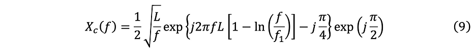
which can further be simplified as:

Similar to the process of deconvolution with the Synchronized Sine-Sweep, the division of Yc(f) by Xc(f) defined above is an effective method for deconvolution for the Synchronized Cosine-Sweep.
It is also worth noting that different definitions for xc(t) and Xc(f) are defined by Novak in [4], but yield less than desirable outcomes during implementation. If a synchronized cosine sweep is needed, it is recommended to instead use equations (8) and (10) above.
Chapter 3: The Chebyshev Non-Linear Model
3.1 Chebyshev Polynomials of the First Kind

Figure 6: Graph of Chebyshev Polynomials of the First Kind, up to the 5th order.
Chebyshev Polynomials of the First Kind are a series of polynomials closely related to the cosine function. A kth order Chebyshev Polynomial, Tk(x), is defined with the following identity:

These polynomials are shown expanded below, up to the 5th order:

because of the identity in equation (11), these correspond to the multiple angle expansions of cos(kθ), shown below:

By looking at the definitions above, it may become apparent why using Chebyshev Polynomials would be useful for modeling harmonics of a signal—as the harmonics cos(kθ) can be created with simple operations on the fundamental signal, cos(θ). This is discussed more in detail in the next section, 3.2.
Like many other polynomial series, Chebyshev Polynomials are also capable of approximating non-linear functions. This is normally done with the summation of increasingly higher-order polynomials, each with a multiplier that needs to be determined. For example, (fig. 7) below shows a simple 5th order Chebyshev approximation of a hyperbolic tangent function (tanh(x)), meaning that the first 5 Chebyshev polynomials each with their own multiplier are added together to create a line resembling the non-linearity. In this case, the coefficients were determined using the Least Squares method to find a line of best fit, but other techniques could be applied.

Figure 7: 5th Order Chebyshev Approximation of tanh(x)
Intuitively, a kth order approximation of any non-linearity can only create harmonics up to the kth order of the input signal; so, a 5th order Chebyshev approximation of tanh(x) can only create up to the 5th harmonic of x. The more polynomials Tk(x) that are used for the approximation, the more accurate it becomes—and in turn, more harmonics can be created.
3.2 The Chebyshev Model
Now that the concept of non-linear modeling with Chebyshev Polynomials has been introduced, one can look into the process of reconstructing an unknown non-linearity with the assistance of the Synchronized Swept-Sine Method outlined in chapter 2. We call this the Chebyshev Model, which is depicted below in (fig. 8); and as we will see, these polynomials are extremely effective with this method due to its unique properties.
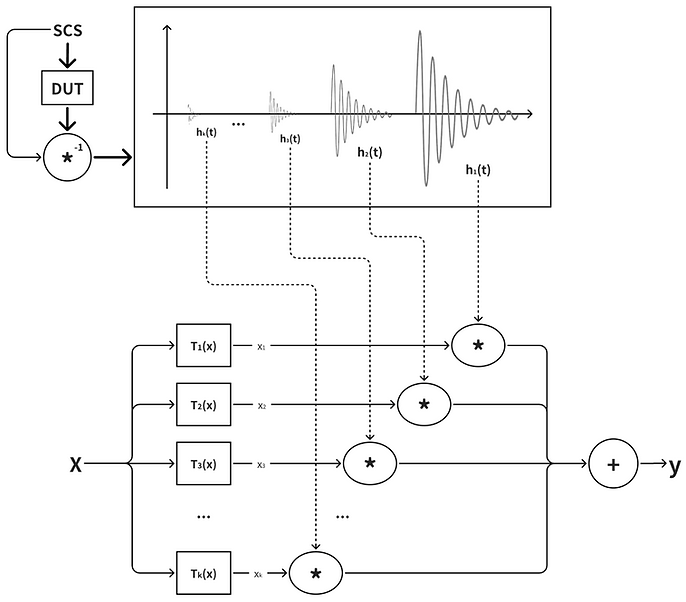
Figure 8: The Chebyshev Non-Linear Model
At first glance, the Chebyshev Model shown above looks similar to the Simplified Non-Linear Volterra Model outlined in Bennett’s paper [11], but with some key differences. With the Chebyshev Model, a Synchronized Cosine Sweep (denoted SCS) is sent through the device under test, and the output is then de-convolved with the original excitation signal. As discussed in chapter 2, this results in a sequence of impulse responses (IRs) of descending order separated by a time gap, each containing data corresponding to their individual harmonic. The information captured in each IR is traditionally processed using a “Mixing Matrix,” where the harmonic data is converted into coefficients for power operators (x^2, x^3, x^4 … ) to process a digital sample. This mixing matrix is often necessary since a specific power operator (e.g. x^7) will contribute to multiple harmonics (7th, 5th, 3rd, and 1st harmonic), and the mixing matrix will essentially calculate how much each power operator contributes when considering all harmonics present and assign a coefficient.
However, the use of Chebyshev Polynomials eliminates the need for a mixing matrix entirely; instead, each impulse response created by the Synchronized Swept-Sine Method can be directly convolved with the digital signal Tk(x) of the respective order. In other words, the impulse responses can be implemented directly as FIR filters for the model without any additional processing (For real-time applications, the IRs can be implemented as common-pole parallel filters rather than FIR filters for computational efficiency, as outlined in [7]).
To understand why this is possible, one can look to Novak’s explanation in his paper [4] where he explains how the identity stated in equation (11) allows for the Chebyshev polynomials Tk(x) to represent a “generator” producing pure kth higher harmonics when excited with a signal cosωt. So, when given cosine sweep xc(t) as an input, the Chebyshev Polynomial Tk(xc(t)) generates a copy of the sweep with instantaneous frequency k-times higher than the original. This is also why a Synchronized Cosine Sweep must be used for the Chebyshev Model rather than a sine sweep, as the phase difference would prevent the ability to directly convolve the HHIRs.
To determine the operators needed in (fig. 8) during implementation, the following iterative equation can be used to determine the Chebyshev Polynomial operators Tk(x):

where k is a whole number and the degree of the polynomial expression, ⌊x⌋ is a floor function, and is a binomial coefficient. As an example, the third order Chebyshev Polynomial (k=3) can be expanded with this equation, yielding T3(x) = 4x^3 - 3x in accordance with equation (12d). Its respective block diagram for processing a digital sample is shown below in (fig. 9):
( )
n
k

Figure 9: Third-Order Chebyshev Operations
This takes the place of the process block labeled “T3(x)” in (fig. 5)—and similarly, all other kth order definitions of Tk(x) shown in the figure can be found with the same equation.
Now a non-linearity can be effectively modeled, as shown below in (fig. 10):

Figure 10: Approximation of an asymmetric non-linearity using a 20th order Chebyshev Model, and 128-sample FIR filters. Input/Output is curve shown on the left, and waveshape for a 1kHz signal is shown on the right.
In this example, the Synchronized Cosine Sweep was run through a non-linearity defined with a tanh(3x) function for positive values, an atan(3x) function for negative values, and a scaling factor to keep the output signal between -1 and 1. This non-linearity was made intentionally asymmetric to ensure the presence of both odd and even harmonics, and will be used as the example non-linearity for the entire paper unless stated otherwise. The first 20 impulse responses (h1 to h20) from the resulting output were extracted as 128 samples each, and then directly implemented as FIR filters for the signal Tk(x) of corresponding order in the Chebyshev Model. The input/output curve of the estimation was then measured for all sample values between [-1,1], and is shown compared to the original function on the left of (fig. 10). A 1kHz test sine wave was then run through both nonlinearities, and the resulting waveshape comparison is shown on the right. It is worth mentioning that the 128-sample length of each impulse response was determined using trial and error, and the implementation of IRs longer than 128 samples somehow yielded less desirable results. Not much of an explanation was found, other than the possibility of the IR components overlapping as the sample length increases.
Although this method is practically effective for lower orders, issues with underflow start to arise with higher order polynomials due to the increasingly large exponential operations in Tk(x). Performing a large exponential operation on a digital sample within the range of [-1,1] could result in a considerably small value, which could be susceptible to rounding errors and result in the model losing precision. These rounding errors manifest as random noise, subsequently increasing the noise floor of the signal. This problem, typically referred to as “underflow,” becomes increasingly more significant as the exponential operations get larger, since the resulting values become smaller. Fortunately, an alternate method of implementing the Chebyshev Polynomials recursively allows for the minimization of this issue.
The recursive identity for Chebyshev Polynomials is as follows:

where k is a whole number. Defining the polynomials Tk(x) using this recurrence relation rather than explicitly using equation (14) results in a more precise model, as it avoids the use of any exponential operators entirely—which minimizes calculations with extremely small numbers susceptible to rounding errors. A block diagram for a 4th order recursive Chebyshev Model is shown below:

Figure 11: A 4th Order Recursive Chebyshev Model
The recursive model proves to be effective in reducing the noise floor, as shown here:

Figure 12: Noise Floor for both a 55th order Iterative (left) and Recursive (right) Chebyshev Model
In this figure, the left-hand side shows a 1kHz test frequency being run through a 55th order Iterative Chebyshev Model estimating the same asymmetric non-linearity. Here, you can see the noise floor gets as high as -40dB at certain frequencies, completely masking many of the harmonics introduced by the system. The right-hand side of the figure shows the exact same scenario, except a 55th order recursive Chebyshev model is used instead. Here, the noise floor is around -100dB at its highest, which is a reduction of about -60dB. These models were developed in MATLAB, which by default uses double-precision floating-point numbers (more commonly known as doubles) for most computations. Thus, the exact performance of the models may differ when handling mathematical operations with single-precision floating-point numbers, which are far more prevalent in real-time digital audio applications due to their faster processing speeds and lower memory requirements.
3.3 Further Testing
To further measure the effectiveness of each model, a simple test for Root Means Square Error (RMSE) can be performed. In this assessment, the cosine sweep xc(t) is first run through the original non-linear system, generating an output yc(t) that will serve as the benchmark in this comparison. The cosine sweep is then run through both the Chebyshev Iterative and Recursive Models, generating outputs yi(t) and yr(t), respectively. The RMSE can then be found between the benchmark yc(t) and the Chebyshev approximations yi(t) and yr(t) using the rmse() function in MATLAB, with the goal being to achieve as low of an RMSE value as possible. Using the cosine sweep as the input is effective in this case since it allows for a comparison of all frequencies up to Nyquist (2Hz to 24kHz).
After performing this test, both models prove to be extremely accurate at lower orders. The 20th order (20 harmonics) Iterative and Recursive Model both yield an RMSE of 0.0114 when compared to the benchmark, which is a very desirable outcome. This RMSE value holds up until around the 50th order, where the underflow issues start deteriorating the Iterative Model. These issues reach an unacceptable level around 55-60 harmonics, where the RMSE value exceeds 50. The Recursive Model, on the other hand, has no issue dealing with the higher-order harmonics; as shown below in the table, an 100th order estimation raises its RMSE value by only 0.0001. Again, these numbers may vary when using single-precision floating point arithmetic.

It is also worth noting that the Recursive Model performs these tasks considerably faster, taking only 0.82 seconds to complete an 100th order estimation in MATLAB when given a 9.4 second input signal. This is a significant improvement over the Iterative Model, which required 9.07 seconds to complete the same task. Thus, the Recursive Chebyshev Model is a far better choice during implementation.

Regardless of the method, higher-order harmonics will be harder to accurately represent due to the increasingly large number of operations that need to be performed. Even the Recursive Model is susceptible to rounding errors, which simply compound as the order increases. This error will often manifest as small “ripples” at the edges of the input/output curve, which will affect the signal at high amplitudes as shown in the example below.

Figure 13: Distortion of a High Amplitude Signal from a 100th Order Recursive Model
Another evaluation method of the Chebyshev Model involves plotting the frequency response deviation between the benchmark yc(t) and the recursive approximation yr(t), which gives a better idea as to which frequencies are being accurately represented. In this case, a 20th order Recursive Chebyshev Model is used to approximate both a linear system with no introduced harmonics on the left, and the asymmetric non-linearity created before in (fig. 10) on the right.

Figure 14: Frequency Response of a Chebyshev Approximation of a linear system (left), and a non-linear system (right) in Comparison to the original DUT.
The figure above illustrates that the difference in frequency response between the benchmark and the Chebyshev Model is minimal, further indicating that the two outputs are extremely similar. Nevertheless, the Chebyshev Approximation starts to show some amplitude differences at higher frequencies, with the worst error being around a 2.5dB difference around Nyquist for the linear system, and nearly a 30dB difference in the same area for the non-linear system with harmonics introduced. These results seem to stay consistent even if a higher-order Chebyshev Model is used; but thankfully, when using a sample rate of 48000, the error falls beyond the audible hearing range for humans and can be filtered out using a lowpass filter.
Chapter 4: Anti-Derivative Anti-Aliasing
4.1 Aliasing and Alias Reduction
Aliasing distortion is a common problem in digital audio. As a review, digital formats are only capable of accurately representing frequencies up to half of the sampling rate; so for a digital audio file with 48,000 samples per second, 24kHz is the highest possible frequency it can accurately represent. This limit is formally known as the “Nyquist Frequency.” If a frequency higher than Nyquist is introduced, such as a harmonic from a non-linearity, an incorrect frequency lower than Nyquist will be introduced in the signal due to the inaccurate representation, which is often unpleasant and within the audible hearing range. This error is called aliasing, and a simple visualization of the concept is shown below in (fig. 15).
Intuitively, this means that aliasing does not occur with analog audio systems where the signal is represented in continuous time, since it can be thought of having an infinitely high sampling rate—and thus an infinitely high Nyquist frequency.

Figure 15: Example of Aliasing
A common solution to combat aliasing is by simply increasing the sample rate of the digital audio signal to push the Nyquist frequency higher. This method is also known as oversampling, which effectively reduces the issue since many aliased frequencies will start to become higher than the limit of human hearing. In addition, the harmonics introduced by a non-linear system commonly tend to decrease significantly in amplitude as they increase in frequency, meaning that any frequencies that exceed Nyquist may be considerably quieter anyway when increasing the sampling rate. Although oversampling is extremely effective, this method may not always be practical since it is computationally expensive, and many digital systems do not support higher sampling rates in the first place. Thus, other methods for anti-aliasing must be explored.
The concept of Anti-Derivative Anti-Aliasing (ADAA) was first introduced by Julian Parker et al. in [14], and outlines an alternate approach of reducing aliasing that arises from a digital non-linear system. As an overview, the ADAA method is performed by first creating a continuous-time version of the signal using interpolation between samples, then applying the non-linearity and a lowpass filter in continuous time to reduce aliasing, and finally converting the signal back to discrete-time at the original sample rate. The paper offers a simple general formula for this process, and a brief summary of the derivation is shown below.
To start, the continuous-time approximation x̃(t) of the digital input signal x[n] is created with linear interpolation between samples, which can be written as:

where τ = 1 - (t mod 1), a time variable that runs between each sample. Parker describes how higher-order interpolation would theoretically result in a better estimation of the signal and yield a better result, but using linear interpolation is used as it allows for a general equation to be derived. With this continuous-time signal x̃(t), the output of the non-linear function f(x̃(t)) can now be found for any value of t; and this continuous-time output can be notated as y(t). To reduce aliasing, however, some sort of filtering must be applied to y(t) to minimize frequencies above Nyquist before it is sampled and converted back to a digital signal. In other words, applying a lowpass filter in continuous time allows for the reduction of high frequencies before they alias. In comparison, if the signal is not converted to continuous-time and a non-linearity is applied, the frequencies above Nyquist that are introduced will simply be reflected into the frequency range of the non-aliasing harmonics we want to keep; and thus, they cannot be filtered out separately.
In this case, a simple rectangular filter kernel is applied to y(t) to reduce aliasing using continuous-time convolution, yielding:

where ỹ(t) is the filtered continuous-time output, and hrect is a function of unit width:

which means ỹ(t) can be expressed more simply:

An expression for the digital output y[n] can then be found, since y[n] = ỹ[n], yielding:

Since only the range from 0 to 1 is being considered, one may notice that u = τ, meaning we can rewrite the equation to the following:

and with integration by substitution:

As explained in Parker’s paper, the linear interpolation between samples in x̃ becomes useful here since dx̃/dτ is constant in this case, and can be factored out of the integral. The expression can now be written as:

This can then be further simplified to give us the final Anti-Derivative Anti-Aliasing equation:

where F1 is the anti-derivative of the function, f. Using a rectangular filter kernel of unit width defined in equation (18) allows for the derivation of a simple ADAA equation as shown above; however, the limitation is the frequency response of the filter. The use of a higher-order kernel such as a triangular filter will result in more effective suppression of frequencies above Nyquist, but complicates the equation significantly. Therefore, for the purposes of this paper, we will employ the simpler method using a rectangular filter kernel.
4.2 Iterative ADAA Method for the Chebyshev Model
With ADAA processing, the Iterative Chebyshev model is modified; each process block containing a Chebyshev polynomial (T1(x),T2(x) … Tk(x)) is replaced with an ADAA block of corresponding degree (ADAA1(x), ADAA2(x) … ADAAk(x)), as shown in (fig. 16):

Figure 16: A Modified Iterative Chebyshev Model to support ADAA
To determine the operations needed for each new ADAA block, a general equation for anti-derivative anti-aliasing can be derived by modifying the Chebyshev polynomial formula. If the equation of Tk(x) defined in equation (14) is set as the function f, then its anti-derivative, F1(x), can be defined with the following:

This can be simplified greatly by temporarily substituting the part of the equation determining the coefficient with an arbitrary placeholder variable. By doing so, F1(x) can now be expressed as:

where B is defined as:

The definition of the anti-derivative F1(x) can now be plugged into the ADAA formula from equation (24), yielding:

To ensure stability of the model, the x terms in the denominator must be canceled out since a denominator of zero will return an infinitely high value, and near-zero denominators will be significantly affected by rounding errors. Fortunately, the x terms in our numerator form a difference of two squares, which allows for the factorization of a matching term.

The denominator can now be canceled out, yielding:

Our arbitrary placeholder variable can now be substituted with its original expression, resulting in the final iterative Anti-Derivative Anti-Aliasing Chebyshev equation.

Using this equation, each ADAA process block can be determined. For demonstration purposes, the third order anti-derivative anti-aliasing equation (ADAA3) is expanded below, and its block diagram is depicted in (fig. 17).


Figure 17: Third-Order ADAA Operations for the Iterative Chebyshev Model
This block diagram the place of the ADAA3(x) process block shown in (fig. 16), and all other order ADAA process blocks can be determined by using equation (30).
4.3 Recursive ADAA Method for the Chebyshev Model
Alternatively, the Chebyshev ADAA equation can be defined recursively rather than explicitly. This is made possible by the following identity for the integration of Chebyshev Polynomials defined in [6]:

where F1(x) is the anti-derivative of Tk(x), and k ≥ 2. With this definition above, we can substitute can substitute F1(x) into the ADAA general formula (equation (24)) shown earlier, yielding:

Which can then be further simplified to give us our final Recursive ADAA Chebyshev equation:

This equation can only be used for values of k ≥ 2, which means a definition for ADAA0 and ADAA1 must be found explicitly. This can be done using the Iterative Chebyshev ADAA formula from equation (30), or by plugging the anti-derivatives of T0(x) and T1(x) straight into the general ADAA formula eq. (27). This direct approach is shown below with T0(x), whose anti-derivative is defined simply as F1(x) = x. This results in the derivation of ADAA0 being:

The same process can be used for T1(x), which results in ADAA1 being defined as:

Similarly to the non-ADAA Recursive model, this method is beneficial in reducing underflow issues that may arise with defining ADAAk explicitly as it avoids the use of exponential operators. The drawback is that the x term in the denominator of equation (34) cannot be canceled out; and as previously mentioned, a near-zero denominator will be significantly affected by rounding errors, which could result in a wildly incorrect value. Thus, an escape clause must be created during implementation for small values of the denominator, with the most straightforward approach being to revert to the first order equation defined with equation (36). The series of equations defining ADAAk≥2 now becomes:

where the value of TOL is defined to best fit the situation. Thus, the choice between an Iterative or Recursive ADAA model during implementation is less clear than its non-ADAA counterpart. On one hand, the Iterative ADAA model is stable since the derivation allows for the cancelation of the x terms in the denominator, but is considerably more computationally expensive and suffers underflow issues at higher orders. On the other hand, the Recursive ADAA model addresses the underflow issues and is overall more computationally efficient, but the model is not stable and needs an escape clause during implementation.
4.4 Results
Using the ADAA method effectively reduces the amplitude of aliasing frequencies in both the Iterative and Recursive Chebyshev Models; and as expected, applying ADAA yields the same result for both, so only the Iterative ADAA Model will be used to demonstrate for this section. To ensure there is truly no difference, the cosine sweep was run through both a 40th order Iterative and Recursive model approximating the same non-linearity to ensure all frequencies and possible aliasing were considered, and the resulting RMSE value comparing the two outputs was 8.2e-13; irrefutably negligible.
(Fig. 18) below shows a spectrogram of the resulting output of a cosine sweep being run through both a 40th order non-ADAA and ADAA Chebyshev model, which are both approximating the asymmetric non-linearity used before. The straight lines traveling upwards represent the cosine sweep and its harmonics, and the curved lines reflecting off the top represent aliasing.

Figure 18: Spectrogram of Chebyshev Approximations of an Asymmetric Non-Linearity; one without ADAA (left), and one with ADAA (right)
In this figure the left-hand side represents the Chebyshev approximation with no Anti-Aliasing, while the right-hand side represents the Chebyshev approximation with ADAA; and as shown, the ADAA Chebyshev model has considerably less energy in the aliasing frequencies, while maintaining the energy in the harmonics. However, one can see that some additional ultra-low frequency error (near DC) is produced in the bottom right corner of the ADAA spectrogram, which seems to show up whenever there are even harmonics present. The figure below shows a similar comparison with a symmetrical non-linearity, which only produces odd harmonics; and in this case, the ADAA version does not have the low-frequency discrepancy.

Figure 19: Spectrogram of Chebyshev Approximations of a Symmetric Non-Linearity; one without ADAA (left), and one with ADAA (right)
To better understand the characteristics of the error, a shorter cosine sweep starting from a higher frequency can be used as an input to the model—meaning that any low frequency content present in the output would be due to the error, which can then be isolated and studied. The figure below shows the resulting graph of the experiment for low frequencies, which suggests that the error starts around 20-30Hz and increases in amplitude as the frequency decreases towards DC.

Figure 20: Low-Frequency Error in the ADAA Model with Even Harmonics
Although the underlying cause remains unclear, the error is fortunately low enough in frequency to where it can be addressed with a gentle high-pass or low-shelf filter with cutoff around 20 or 30Hz. This would be particularly effective in this case, as the attenuation of the filter would be complementary to the frequency characteristic of the error; and will not have much effect on the signal around the cutoff where important frequencies in the low-end of certain instruments may be. This solution could be expanded further to address the problem more effectively by implementing multiple high pass filters with increasing cutoff frequencies, with respect to the increasing harmonics as shown below in (fig. 21). This would theoretically prevent any unneeded frequency content from reaching the output, avoiding any possible accumulation of error.

Figure 21: Potential Solution for the Low Frequency Error
Although this method could potentially eliminate the low-frequency error entirely, further research is needed to determine the precise cutoffs for each filter and to evaluate its effectiveness when compared to using a single high-pass filter at the output. The cutoff of each filter using this method could theoretically be increased by a multiple of k for each harmonic, since the kth harmonic would be a kth multiple higher-frequency copy of the original signal. In other words, the signal in each parallel branch of the model would have less low-frequency content than the previous one, and could be filtered even more. For example, if the lowest frequency in the original signal is 20Hz, then a suitable cutoff frequency of for a high-pass filter in the first branch would be around 20Hz since it represents the fundamental signal. Intuitively, this means that the lowest frequency in the second harmonic would be 40Hz, meaning that anything lower would be irrelevant and can be filtered out; and thus, the cutoff for the filter in the second branch could be around 40Hz. The lowest frequency in the 3rd harmonic would be 60Hz, meaning that the third high-pass filter could be set around 60Hz, and so on. Following this method could result in a considerably more accurate model, as any frequencies lower than each harmonic would be filtered out—leaving no room for error. However, this is just a simple fix; finding the root cause of the error would prove to be more beneficial, as it could lead to the development of a completely different method to address the issue with greater efficiency.
To further measure the performance of the ADAA method with the Chebyshev model, a simple test can be conducted by first starting with a high-frequency test signal (5kHz, for example) and running it through both a non-ADAA and ADAA Chebyshev approximation of the asymmetric non-linearity. 5kHz is used in this case to ensure aliasing occurs, and the asymmetric non-linearity is used to ensure the presence of both even and odd harmonics. The level of each aliasing frequency can then be measured in both models, from which an average alias attenuation can be found. In this example a sampling rate of 48000 samples per second is used, so the Nyquist frequency is 24kHz.

The table above shows the first 20 harmonics of the 5kHz tone, with the last 16 entries being the aliasing frequencies. The average alias attenuation achieved is 16.26dB, which proves the ADAA method is effective in reducing aliasing. This measured alias reduction also stays consistent with the application ADAA to the Volterra Model in Bennett’s paper [11], which had a mean 17.0dB reduction for the first 16 alias locations—implying that the ADAA method provides a similar result for any application.
As table 4 suggests, the rectangular filter kernel used in the ADAA equation also imparts a slight lowpass characteristic on non-aliasing frequencies below Nyquist as well. This is not ideal, but unfortunately is unavoidable. The lowpass characteristic can be graphed with a special method, which is achieved by first creating cosine sweep xc(t) from 2Hz to Nyquist, and running it through the non-ADAA and ADAA Chebyshev approximations of a linear system, y = x. Using this linear function ensures that no harmonics of the signal are created, which in turn ensures that only frequencies below Nyquist are considered. The frequency response of both models can then be found by taking the FFT of each, and difference between the two results in the graph shown below. As one can see, the frequencies below Nyquist are noticeably attenuated, with frequencies as low as 10kHz being reduced by about -2.5dB.

Figure 22: Frequency Response of the ADAA Method below Nyquist
However, this graph also suggests that the non-aliasing frequencies at 15kHz and 20kHz should be attenuated by around -5dB and -12dB, respectively, which from the table we can see is not the case. Not much of an explanation was found here, and may suggest a discrepancy in the implementation.
A simple RMSE test can also be performed to validate that the utilization of the ADAA method does not make the Chebyshev Model less accurate. When considering a 1kHz test sine tone being run through both a non-ADAA and ADAA Chebyshev approximation of the asymmetric non-linearity, the rmse() function in MATLAB returns a value of 0.0627, suggesting a negligible error introduced by the ADAA method. When comparing the ADAA Chebyshev Model the original device under test, the rmse() function returned a value of 0.0639.

Figure 23: Comparison of Waveshape between the Original Non-Linearity and the ADAA Chebyshev Approximation
Since the goal of this test was to determine if the ADAA method has an overall negative effect on the waveshape, 1kHz was chosen as the test frequency to ensure minimal aliasing. Choosing a higher frequency with significant aliasing would not be effective in this case, since the waveshape would change purposefully in the ADAA method to reduce aliasing, and thus result in a higher RMSE value.
In addition to the underflow issues, the primary limitation of the Iterative ADAA method lies in the significant increase of operations, which drastically reduces computational efficiency and makes higher-order iterative models impractical for use beyond a testing environment. Even when considering as few as 20 harmonics, the Iterative ADAA model required 4.42 seconds to process a 9.4 second signal—a task completed in just 0.4 seconds without ADAA. The computation time quickly became unacceptable with higher order models, as raising the number of harmonics to 45 resulted in a computation time of 46.8 seconds, compared to only 1.79 seconds without ADAA. On the other hand, the Recursive model suffered much less when ADAA was applied. Although there was an increase in computation time it was considerably more manageable, with an 100th order model taking only 2.8 seconds to process a 9.4 second signal. Thus, the Recursive model must be used if the application of ADAA is desired for any real-time processing.

Chapter 5: Conclusion and Further Research
As discussed in this paper, utilizing a cosine sweep for the Synchronized Swept-Sine Method in combination with the Chebyshev Non-Linear Model serves as an effective method for modeling an unknown non-linearity, such as a guitar amplifier or distortion pedal. Although the signal may suffer issues with aliasing due to the harmonics introduced above the Nyquist frequency, applying the ADAA method to the Chebyshev Model successfully reduces the energy of aliasing frequencies by about 16dB, yielding similar results as when previously applied to the Volterra Non-Linear Model shown in [11]. This paper defines a general equation for the ADAA Chebyshev Model both iteratively and recursively; and although they both have their benefits and shortcomings, the Recursive model proves to be the far better choice for any real-time application due to its computational efficiency.
Future research could begin by addressing the issues outlined in this paper. Firstly, a deeper examination into why the Chebyshev Model yielded less desirable results when increasing the length of each IR longer than 128 samples during implementation would be insightful. This finding is counterintuitive and may indicate an implementation error, as a longer-length impulse response typically enhances resolution of a filter rather than degrading it. As discussed in Chapter 3, this may be caused by a slight overlap in the IRs, which would theoretically become more problematic as the sample length increases; however, it is possible that this discrepancy could be due to a different issue entirely. Furthermore, implementing these impulse responses as common-pole parallel filters instead of FIR filters could significantly improve the model's computational efficiency as outlined in [7], and may be useful especially if a real-time application of the model is desired. The high-frequency estimation error near the Nyquist limit in the Chebyshev Model as illustrated in (fig. 14) should also be examined further, particularly because it remains unexplained. While this error is not problematic at higher sampling rates since it resides above the audible frequency range, it could become an issue at lower sampling rates where it would fall within the audible spectrum. Finally, the low-frequency error introduced by the ADAA method should be addressed as well; and exploring the proposed solution of multiple high-pass filters with varied cutoff frequencies, as shown in (fig. 21), could be a viable solution. As discussed in chapter 4, this alternate method would filter out any unneeded frequency content before it reaches the output, which would eliminate any buildup of low-frequency error and result in a more accurate model.
Beyond these issues, plenty of research can be done to further widen the scope of this project. This can include the use of a higher-order filter kernel in the ADAA method for the better suppression of aliased frequencies as outlined in [14], such as a triangular or 2nd order rectangular kernel. These will be more effective in in reducing aliasing when compared to the simple rectangular kernel of unit width implemented in this project, but unfortunately may also lead to a greater attenuation of the high frequencies below Nyquist. The resulting final equations using these higher-order kernels would be far more complex as well, which could pose a challenge during implementation. Furthermore, the ADAA method could be applied to different non-linear models entirely, such as the Legendre Model proposed by Hopman in [12]. This could be particularly useful as it would allow for a comparison of the alias reduction, potentially reinforcing the notion that the ADAA method yields consistent results across various contexts. Most importantly, developing a definition for the ADAA Recursive Chebyshev Model that omits any x term in the denominator would be extremely valuable in further research, as it would allow for a completely stable and computationally efficient model ready for real-time digital audio applications.
References
[1] A. Novak, P. Lotton, and L. Simon, “Synchronized Swept-Sine: Theory, Application and Implementation,” J. Audio Eng. Soc., vol. 63, no. 10 (2015 Oct.). doi: http://dx.doi.org/10.17743/jaes.2015.0071
[2] C. Bennett, “Digital Audio Theory: A Practical Guide” (2020 Dec.). https://digitalaudiotheory.com/dat
[3] A. Novak, L. Simon, P. Lotton, and F. Kadlec, “Modeling of Nonlinear Audio Systems using Swept-Sine Signals: Applications to Audio Effects,” in Proc. of the 12th Int. Conference on Digital Audio Effects (DAFx-09), Como, Italy, September 1-4, 2009. https://www.researchgate.net/profile/Antonin-Novak-2/publication/228860165_Modeling_of_Nonlinear_Audio_Systems_using_Swept-Sine_signals_Application_to_audio_effects/links/0fcfd5086a31d19854000000/Modeling-of-Nonlinear-Audio-Systems-using-Swept-Sine-signals-Application-to-audio-effects.pdf
[4] A. Novak, L. Simon, P. Lotton, and J. Gilbert, “Chebyshev Model and Synchronized Swept Sine Method in Nonlinear Audio Effect Modeling,” in Proc. of the 12th Int. Conference on Digital Audio Effects (DAFx-10), Graz, Austria , September 6-10, 2010. doi: https://www.dafx.de/paper-archive/2010/DAFx10/NovakSimonLottonGilbert_DAFx10_P23.pdf
[5] E. Weisstein, “ Chebyshev Polynomials of the First Kind,” From MathWorld–A Wolfram Web Resource. https://mathworld.wolfram.com/ChebyshevPolynomialoftheFirstKind.html
[6] “Chebyshev polynomials” From Wikipedia, The Free Encyclopedia. https://en.wikipedia.org/wiki/Chebyshev_polynomials
[7] B. Bank, “Computationally Efficient Nonlinear Chebyshev Models Using Common-Pole Parallel Filters with the Application to Loudspeaker Modeling,” (2011 May.).
https://www.aes.org/e-lib/browse.cfm?elib=15883
[8] A. Novak, L. Guadagnin, B. Lihoreau, P. Lotton, E. Brasseur, and L. Simon, “Measurements and Modeling of the Nonlinear Behavior of a Guitar Pickup at Low Frequencies,” (2017 Jan.). https://www.mdpi.com/2076-3417/7/1/50
[9] A. Novak, L. Simon, and P. Lotton, “Extension of Generalized Hammerstein Model to Non-Polynomial Inputs,” (2016 Aug.). https://ieeexplore.ieee.org/document/7760202
[10] M. Reed and M. John Hawksford, “Practical Modelling of Nonlinear Audio Systems Using the Volterra Series,” (1996 Jan.).
[11] C. Bennett and S. Hopman, "Antialiasing for Simplified Nonlinear Volterra Models," J. Audio Eng. Soc., vol. 70, no. 9, pp. 690-697, (2022 Sep.). doi: https://doi.org/10.17743/jaes.2022.0033
[12] S. Hopman, “Advances in the Simplified Nonlinear Volterra Model,” (2023 Apr.). https://scholarship.miami.edu/esploro/outputs/other/Stefan-Hopman--Advances-in-the/991031798915302976
[13] S. Arora, C. Bennett, “Fast Algorithms for Black Box Modelling of Static Hammerstein Nonlinearities,” (2022 Oct.). https://www.aes.org/e-lib/browse.cfm?elib=21961
[14] J. Parker, V. Zavalishin, E. Le Bivic, “Reducing the Aliasing of Nonlinear Waveshaping using Continuous-Time Convolution,” in Proc. of the 19th Int. Conference on Digital Audio Effects (DAFx-16), Brno, Czech Republic, September 5-9, 2016. https://dafx16.vutbr.cz/dafxpapers/20-DAFx-16_paper_41-PN.pdf
[15] S. Bilbao, F. Esqueda, J. D. Parker, and V. Välimäki, “Antiderivative Antialiasing for Memoryless Nonlinearities,” IEEE Signal Process. Lett., vol. 24, no. 7, pp. 1049–1053 (2017 Jul.). https://doi.org/10.1109/LSP.2017.2675541.